Differenze tra le versioni di "Calcolo probabilità e statistica matematica/Esami/2008-01-10"
(→Testo soluzione) |
(→Testo soluzione) |
||
| Riga 50: | Riga 50: | ||
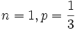
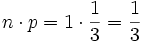
<math> {n \cdot p} = 1 \cdot {1 \over 3} = {1 \over 3}</math> | <math> {n \cdot p} = 1 \cdot {1 \over 3} = {1 \over 3}</math> | ||
| − | <math> {(1-p)^n} = (1 - {1 \over 3})^1 = {2 \over 3}</math> | + | <math> {(1-p)^n} = \bigg (1 - {1 \over 3}\bigg )^1 = {2 \over 3}</math> |
** b) <math>n=10, p={1 \over 30}</math> | ** b) <math>n=10, p={1 \over 30}</math> | ||
| Riga 56: | Riga 56: | ||
<math> {n \cdot p} = 10 \cdot {1 \over 30} = {1 \over 3}</math> | <math> {n \cdot p} = 10 \cdot {1 \over 30} = {1 \over 3}</math> | ||
| − | <math> {(1-p)^n} = (1 - {1 \over 30})^{10} = ({29 \over 30})^{10} = 7,12 \cdot 10^{-1}</math> | + | <math> {(1-p)^n} = \bigg (1 - {1 \over 30}\bigg )^{10} = \bigg ({29 \over 30}\bigg )^{10} = 7,12 \cdot 10^{-1}</math> |
** c) <math>n=10^9, p={1 \over {3 \cdot 10^9}}</math> | ** c) <math>n=10^9, p={1 \over {3 \cdot 10^9}}</math> | ||
| Riga 62: | Riga 62: | ||
<math> {n \cdot p} = 10^9 \cdot {1 \over {3 \cdot 10^9}} = {1 \over 3}</math> | <math> {n \cdot p} = 10^9 \cdot {1 \over {3 \cdot 10^9}} = {1 \over 3}</math> | ||
| − | <math> {(1-p)^n} = (1 - {1 \over {3 \cdot 10^9}})^{10^9} = 7,17 \cdot 10^{-1}</math> | + | <math> {(1-p)^n} = \bigg (1 - {1 \over {3 \cdot 10^9}}\bigg )^{10^9} = 7,17 \cdot 10^{-1}</math> |
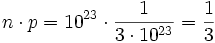
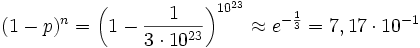
** d) <math>n=10^{23}, p={1 \over {3 \cdot 10^{23}}}</math> | ** d) <math>n=10^{23}, p={1 \over {3 \cdot 10^{23}}}</math> | ||
| Riga 68: | Riga 68: | ||
<math> {n \cdot p} = 10^{23} \cdot {1 \over {3 \cdot 10^{23}}} = {1 \over 3}</math> | <math> {n \cdot p} = 10^{23} \cdot {1 \over {3 \cdot 10^{23}}} = {1 \over 3}</math> | ||
| − | <math> {(1-p)^n} = (1 - {1 \over {3 \cdot 10^{23}}})^{10^{23}} \approx e^{-{1 \over 3}} = 7,17 \cdot 10^{-1} </math> | + | <math> {(1-p)^n} = \bigg (1 - {1 \over {3 \cdot 10^{23}}}\bigg )^{10^{23}} \approx e^{-{1 \over 3}} = 7,17 \cdot 10^{-1} </math> |
| Riga 101: | Riga 101: | ||
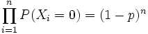
<math>P(S_{m(x)}=0) = P(X_1=0 \land X_2=0 \land ... \land X_{\lfloor x \rfloor}=0) = \prod_{i=1}^{\lfloor x \rfloor} P(X_i = 0) = (1-p)^{\lfloor x \rfloor}</math> | <math>P(S_{m(x)}=0) = P(X_1=0 \land X_2=0 \land ... \land X_{\lfloor x \rfloor}=0) = \prod_{i=1}^{\lfloor x \rfloor} P(X_i = 0) = (1-p)^{\lfloor x \rfloor}</math> | ||
| + | |||
| + | Quindi: | ||
| + | |||
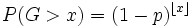
| + | <math>P(G>x) = (1-p)^{\lfloor x \rfloor}</math> | ||
| + | |||
| + | ** b) | ||
| + | <math>F_G(x) = P(G \le x) = 1 - P(G > x) = 1 - (1-p)^{\lfloor x \rfloor}</math> | ||
* punto 4) | * punto 4) | ||
| + | <math>p={1 \over 3} \Rightarrow 1-p = {2 \over 3} \Rightarrow F_G(x) = 1 - \bigg ({2 \over 3}\bigg )^{\lfloor x \rfloor}</math> | ||
| + | |||
| + | NB: Il disegno qui e' un po' un casino da fare, comunque e' quello che si trova sul libro a pag. 67 (figura 2.2), cambiano solo i valori sulle ordinate: | ||
| + | |||
| + | <math>x=1 \Rightarrow F_G(x) = {1 \over 3}</math> | ||
| + | |||
| + | <math>x=2 \Rightarrow F_G(x) = {5 \over 9}</math> | ||
| + | |||
| + | <math>x=3 \Rightarrow F_G(x) = {19 \over 27}</math> | ||
| + | <math>x=4 \Rightarrow F_G(x) = {65 \over 81}</math> | ||
| + | <math>\vdots</math> | ||
ESERCIZIO III | ESERCIZIO III | ||
Versione delle 14:39, 12 gen 2008
Indice
Tema d'esame del 10-01-2007
Problemi modellati
- Generatore di impulsi
Distribuzioni
- Bernoulli
- Binomiale
- Geometrica
Immagine testo

Testo soluzione
ESERCIZIO I
 sono v.c. bernoulliane indipendenti e identicamente distribuite
 con
con 
quindi 
- punto 1)
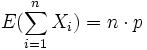
per la linearita' del valore atteso:
e visto che sono identicamente distribuite:
- punto 2)
visto che

e che le X sono indipendenti e identicamente distribuite:
- punto 3)
dal punto precedente abbiamo che:
e che:
- a)
- a)
- b)
- b)
- c)
- c)
- d)
- d)
ESERCIZIO II

sono impulsi BINARI, quindi distribuiti secondo Bernoulli
(NB: Il fatto che i valori che l'impulso puo' assumere siano '1' e '-1' non e' rilevante nel nostro caso, potrebbero benissimo essere '2' e '3' oppure 'a' e 'b', quello che conta qui NON e' QUALI ma QUANTI valori puo' assumere l'impulso, cioe' 2 valori)
- punto 1)

- punto 2)
 "numero di segnali '1' emessi nei primi
  secondi"
 conta il numero di impulsi='1', ovvero conta i "successi"; quindi e' distribuita come una BINOMIALE di parametri
  e
e  .
.
- punto 3)
G = "numero di secondi passati al primo segnale '1'"
quindi G e' distribuita come una GEOMETRICA.
- a)
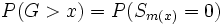
La probabilita' che il primo impulso '1' avvenga DOPO il tempo equivale a dire che tutti gli impulsi fino al tempo son stati '-1', ovvero insuccessi; quindi devo sommare insuccessi.

Quindi:
- b)

- punto 4)
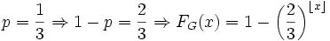
NB: Il disegno qui e' un po' un casino da fare, comunque e' quello che si trova sul libro a pag. 67 (figura 2.2), cambiano solo i valori sulle ordinate:

ESERCIZIO III
- punto 1)
- punto 2)
- punto 3)
- punto 4)
- punto 5)
- punto 6)
Domande orale
--